.png)
Uncertainty is a parameter that must always accompany any measurement of any magnitude, since no measurement is complete without its associated uncertainty. As always, there are many definitions, and they are all facets of the same reality. So let's start with the first. There is a document called GUM (Guide to the Expression of Uncertainty in Measurement) that has become a standard in many countries. For example, in Mexico, it is standard NMX-CH-140-IMNC. This document sets forth the rules and definitions for how uncertainty should be calculated and expressed.
The formal explanation given in this guide (GUM) defines measurement uncertainty as a "parameter associated with the result of a measurement, which characterizes the dispersion of the values that could reasonably be attributed to the measurand." In other words, uncertainty represents the range of values within which the true value of what is being measured is likely to lie.
This definition includes another term that is sometimes little known: "measurand." The measurand is the technical name we use in metrology to refer to the specific quantity we want to measure. It is the objective of our measurement, the "what" we are trying to quantify. For example, if we want to calibrate a scale, then the magnitude is Mass, but the measurand is the Error of Indication of said scale. In the case of a liquid-in-glass thermometer, the magnitude is temperature, but the measurand is the reduced correction (RC). And finally, if we have a flowmeter, the magnitude is flow, but the measurand is the meter factor (MF).
So, returning to uncertainty, this parameter does not indicate error, but rather expresses reasonable doubt about the measured value, taking into account the possible factors of variation in the measurement process. These factors can be intrinsic to the equipment, environmental factors, and factors related to the personnel performing the calibration.
In simpler terms:
Every time we make a measurement, no matter how precise the equipment or how careful we are, there is always a margin of doubt. That is uncertainty. It doesn't mean we've done something wrong or that the equipment is simply damaged; in the real world, conditions are never 100% perfect.
Uncertainty helps us quantify this reality. It tells us that our result is close to the true value, but within a possible range, and it can also be interpreted as a quantitative measure of measurement quality: the lower the uncertainty, the higher the quality.
Now, it's important to know that there are several types of uncertainty, and they can be divided into:
Type A Uncertainty
Type A uncertainty is assessed using statistical methods. Imagine we take the same measurement many times, with the same instrument, under the same conditions. Each time, the results may vary slightly, and those small changes are due to natural random variations in the measurement process. To quantify this uncertainty, we analyze that data using statistics (for example, by calculating the mean and standard deviation).
When we talk about Type A uncertainty, you're basing your analysis on repeatedly observed data. By analyzing the results, you can see how much they vary and use that information to estimate a margin of uncertainty. The more times you repeat the measurement, the more accurate the data you have about those variations will be. This assessment is reliable because it's based directly on practical observations.
In short, Type A uncertainty reflects the variability that can be observed and quantified with statistical methods using repeated data.
Type B Uncertainty
Type B uncertainty is different because it's not assessed through repeated measurements, but rather through other types of information. Here, factors such as previous experience, information provided by the instrument manufacturer, or historical data must be considered. For example, if you have a scale and the manufacturer specifies a margin of error of ±0.1 grams, you use that data as a source of Type B uncertainty.
You can also consider the influence of external factors that you can't directly observe at the time of the measurement, such as estimated environmental conditions or known limitations of the equipment. Type B uncertainty is a combination of expert judgment, specifications, and references, and although it is not based on directly observed data, it is still a valid and well-founded estimate.
In short, Type B uncertainty is uncertainty we estimate based on external information and experience, without the need for repeated measurements.
Now, the above is how uncertainty is classified, but it can also be divided according to which part of the uncertainty process it involves.

Let's explain each type of uncertainty in a little detail:
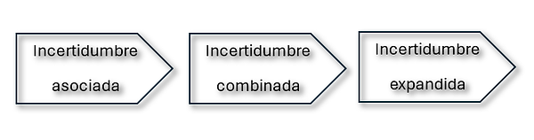
Associated Uncertainty
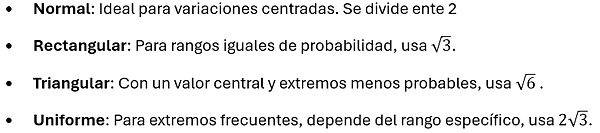
Associated uncertainty is the uncertainty of each component or magnitude of influence that can influence the result of a measurement. When we measure something, several factors can introduce small variations, such as the precision of the equipment or the conditions of the environment. These small variations are represented by probability distributions that reflect the "way" in which these variations occur in each component.
Each distribution has its own "profile" that describes how the measured values are likely to behave, and this affects the associated uncertainty value differently.
Why does distribution matter?
Each distribution has a particular method for calculating uncertainty that suits the nature of the data and best reflects the reality of the measurement process. Choosing the right distribution helps to obtain an accurate and reliable estimate of uncertainty, tailored to how the data behave in practice.
Selecting the correct distribution is key to an accurate and reliable estimation of the associated uncertainty.
As an example, we can say that if we have a scale with a resolution of 0.01 g, the uncertainty associated with that resolution will be uniform, so we have the following:

Combined Uncertainty
Combined uncertainty is the result of grouping or combining associated uncertainties to obtain a total measure of uncertainty of the measurement process. This is done by applying statistical methods, such as "adding" the uncertainties, which is appropriate for independent uncertainties.
Here all the associated uncertainties of each component or influence quantity are taken and a total uncertainty is calculated. The combination is done according to statistical principles to reflect how the uncertainties interact together.
Example: If in a temperature measurement, in addition to the thermometer, other factors intervene such as humidity or the stability of the ambient temperature, the combined uncertainty will be the result of "adding" the associated uncertainties of each of these factors. The sum is not done algebraically, it is done through the law of propagation of uncertainties that is declared by the BIPM (Bureau international des poids et mesures) in the GUM.
Here we enter into another definition that brings with it the same law of propagation, The sensitivity coefficients .
To understand what a sensitivity coefficient is (the partial derivative in the law of propagation) you must first understand that in order to make a good measurement or good calibration, you must have the mathematical model that describes the behavior of that magnitude or measurand. This mathematical model has some variables that are magnitudes of influence, which we already talked about, for example, the resolution, but not all of these variables affect the measurand in the same way, some have more weight than others, so they cannot simply be added together, so it is necessary to know mathematically how much they are affected, normally it is measured as a percentage in an uncertainty budget and it is known as the impact percentage.
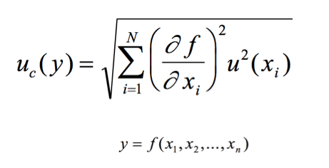
The sensitivity coefficient is calculated by deriving the effect of an input variable on the measurement result. In general, the sensitivity coefficient (ci) for a specific variable is defined as the partial derivative of the measurement function with respect to that variable:

Where:
And it is the result of the measurement (measurand).
Xi is the input variable that influences Y.
This value of ci shows us how much the result (Y) changes with a small variation in Xi.
Step by step to calculate the sensitivity coefficient:
Identify the Measurement Function: First, you need a formula or model that relates the measurement result to the input variables. For example, if you are measuring electrical resistance and you know that it depends on temperature, then your model will include that relationship.
Differentiate with respect to each input variable: Calculate the partial derivative of the measurement function with respect to each variable of interest. This is done by taking the mathematical model and differentiating it with respect to the variable you want to analyze. This gives the sensitivity coefficient ci for that variable.
Evaluate at Measurement Point: If the function includes specific constants or conditions, such as the current ambient temperature or the accuracy of the instrument, use these values to evaluate the sensitivity coefficient under those conditions.
Practical example:
Let's imagine that we are measuring the length (L) of an object which depends on the temperature (T). The relationship between length and temperature is expressed by the following function:
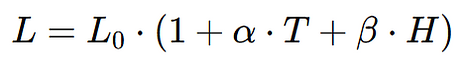
Where:
L0 is the initial length at a reference temperature (e.g. 20 °C).
α is the coefficient of thermal expansion of the material.
β is the coefficient of expansion due to moisture (how moisture affects the length of the material).
To find the coefficient of sensitivity with respect to temperature (cT), we differentiate L with respect to T:
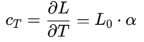
This result shows us that the sensitivity coefficient is equal to the initial length multiplied by the coefficient of thermal expansion. This means that for every degree of change in temperature, the length will vary by this value.
This sensitivity coefficient is then used to adjust for uncertainty. If the temperature uncertainty is, for example, ±0.5 °C (obtained from a calibration certificate), then the effect of this uncertainty on length is calculated by multiplying the sensitivity coefficient cT by the temperature uncertainty. This helps to determine how variation in T influences the measurement result (L). Also multiplying the temperature uncertainty which is in terms of °C by the sensitivity coefficient helps to convert units into terms of the measurand (m).
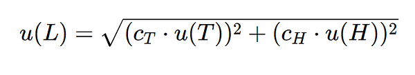
The other sensitivity coefficient of the mathematical model would be the following:
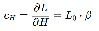
So, having the two coefficients of the model and applying the Law of Propagation of Uncertainties, the combined uncertainty can be calculated as follows:
It should be noted that u(T) and u(H) can propagate independently and may include uncertainties due to certification, resolution, repeatability, drift, etc.
Expanded Uncertainty
Expanded uncertainty is a value that provides an interval within which the true value of a measurement is expected to lie with a specified level of confidence (usually 95%). It is an extension of the combined uncertainty uc, which represents only the standard uncertainty in the measurement, multiplied by a coverage factor k, which widens the range of uncertainty.
The general formula for expanded uncertainty U (capital U) is:
U= uc(y)*k
where k =2.
For a confidence level of approximately 95%, the coverage factor k is typically 2, although this value may vary depending on the effective degrees of freedom.
But what are the effective degrees of freedom?
The effective degrees of freedom ( ν eff) help us to determine the coverage factor k when the standard uncertainties of the input components have different degrees of freedom, for example in measurements with different sources of uncertainty or in small samples (sample). These degrees of freedom are calculated using the Welch-Satterthwaite method:
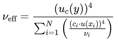
where:
uc(y) is the combined uncertainty.
ci is the sensitivity coefficient of the variable xi.
u(xi) is the standard uncertainty of xi.
νi are the degrees of freedom of each uncertainty component.
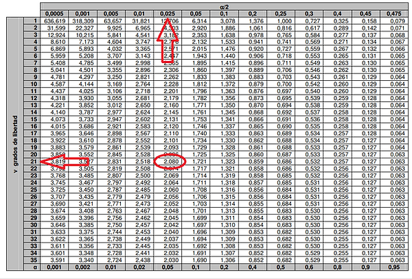
Once ν eff is calculated, a Student t table is used to determine the coverage factor k corresponding to the desired confidence level and effective degrees of freedom.
The degrees of freedom (Vi, differentiated from effective degrees of freedom) are assigned for each uncertainty component based on the way in which that uncertainty has been estimated.
For statistically evaluated uncertainties (Type A), degrees of freedom are assigned based on sample size. In this case:
If you have n observations of a measurement, the degrees of freedom are Vi=n−1
This is because when we calculate a standard deviation from a sample, we lose a degree of freedom (because calculating the sample mean uses one of the data).
Example: If you have 10 measurements of a length and you calculate the standard uncertainty of the mean u(x) of these measurements, the associated degrees of freedom will be Vi=10−1=9.
For uncertainties assessed by non-statistical methods (Type B), the assignment of degrees of freedom is less straightforward. In this case, the value is estimated based on your confidence and knowledge about the source of uncertainty.
Rectangular (Uniform) Distribution: If the uncertainty comes from a source with known limits (e.g. an instrument with a stated accuracy of ±MPE), a high value of degrees of freedom is usually assigned, since there is greater confidence in the accuracy of the estimate (e.g. between 50 and 100 degrees of freedom). This depends on the experience of the metrologist and the knowledge of the equipment.
Normal or Gaussian Distribution: When there is enough information to assume that the value is normally distributed, a high value for degrees of freedom can be assigned. If you do not have precise data, a common value is between 20 and 30 degrees of freedom.
Triangular Distribution: If the value is more concentrated around a point (with less defined limits), an intermediate number of degrees of freedom is usually used, generally between 10 and 20.
Once the degrees of freedom have been assigned and the effective degrees of freedom calculated using the Welch-Satterthwaite equation, we will apply the T-Student table, example:
If in the Welch-Satterthwaite calculation we obtained Veff= 21, that is, 21 effective degrees of freedom, then we will go to the T-student Table and look for the value that corresponds to 21 effective degrees of freedom and a confidence of 95% or what is the same α/2= 0.025, then it gives us a value k=2.080, to be able to multiply it by the combined uncertainty and thus be able to expand it.
So:
U= uc(y)*k
where k =2.08.
In most cases, the t-distribution tables are for 95% probabilities; however, in metrology, a confidence level of 95.45% is used, which completely changes the coverage factor (k). Therefore, it is more advisable to calculate the inverse of the t-distribution using software or Excel (=INV.T.2C(1-0.9545,21)), which gives us k = 2.13. Care must be taken when choosing the probability to be used. The following table is a representation of the t-distribution table for a 95.45% coverage factor:

However, the GUM not only mentions how to calculate uncertainty, but also how to express it. Uncertainty must be expressed in a clear and standardized way to ensure that the results are understandable and useful. It establishes several guidelines for expressing uncertainty so that other users can interpret the results in a consistent manner.
Example of a length measurement with these details:
Result: y=10.0 mm
Combined standard uncertainty: uc(y)=0.15 mm
Coverage Factor k=2 (for 95% confidence)
Expanded uncertainty: U= 0.30 mm
It is also valid to use the symbol ± , example:
10.0 mm ± 0.30 mm
The use of the ± symbol is not recommended when using standard or combined uncertainty since the symbol is usually associated with intervals corresponding to high confidence levels.
Uncertainty should be expressed to two significant figures, where possible.
What Are Significant Figures?
Significant figures are the digits in a number that contribute to its precision. In the context of uncertainty, using two significant figures ensures that the reported value is sufficient to understand the variability in the measurement without being excessive.
Example of expression in two significant figures:
±0.013578mm -> ±0.014mm
± 0.123456 mm -> ± 0.12 mm
± 123.7 mm -> ± 12 cm
And this is how, in a few words and summarizing the topic, the uncertainty in a measurement is calculated, so now you can understand that the action of just measuring, by itself, is not enough if it is not accompanied by the most important parameter within metrology, and if you want to know more about metrology, visit our article: